Optimizing a Permutation-Invariant Function
In this example, we explore BayBE’s capabilities for handling optimization problems with symmetry via automatic data augmentation and/or constraint.
Imports
import os
import numpy as np
import pandas as pd
import seaborn as sns
from matplotlib import pyplot as plt
from matplotlib.ticker import MaxNLocator
from baybe import Campaign, Settings
from baybe.constraints import DiscretePermutationInvarianceConstraint
from baybe.parameters import NumericalDiscreteParameter
from baybe.recommenders import (
    BotorchRecommender,
    TwoPhaseMetaRecommender,
)
from baybe.searchspace import SearchSpace
from baybe.simulation import simulate_scenarios
from baybe.surrogates import NGBoostSurrogate
from baybe.targets import NumericalTarget
Settings
Settings(random_seed=1337).activate()
SMOKE_TEST = "SMOKE_TEST" in os.environ
N_MC_ITERATIONS = 2 if SMOKE_TEST else 100
N_DOE_ITERATIONS = 2 if SMOKE_TEST else 50
The Scenario
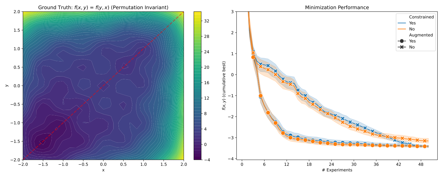
We will explore a 2-dimensional permutation-invariant function, i.e., it holds that \(f(x,y) = f(y,x)\). The function was crafted to exhibit no additional mirror symmetry (a common way of also resulting in permutation invariance) and have multiple minima. In practice, permutation invariance can arise e.g. for mixtures when modeled with a slot-based approach.
There are several ways to handle such symmetries. The simplest one is to augment your data. In the case of permutation invariance, augmentation means for each measurement \((x,y)\) you also add a measurement with switched values, i.e., \((y,x)\). This has the advantage that it is fully model-agnostic, but might come at the expense of increased training time and efficiency due to the larger amount of effective training points.
LBOUND = -2.0
UBOUND = 2.0
def lookup(df: pd.DataFrame) -> pd.DataFrame:
    """A lookup modeling a permutation-invariant 2D function with multiple minima."""
    x = df["x"].values
    y = df["y"].values
    result = (
        (x - y) ** 2
        + (x**3 + y**3)
        + ((x**2 - 1) ** 2 + (y**2 - 1) ** 2)
        + np.sin(3 * (x + y)) ** 2
        + np.sin(3 * np.abs(x - y)) ** 2
    )

    df_z = pd.DataFrame({"f": result}, index=df.index)
    return df_z
x = np.linspace(LBOUND, UBOUND, 25)
y = np.linspace(LBOUND, UBOUND, 25)
xx, yy = np.meshgrid(x, y)
df_plot = lookup(pd.DataFrame({"x": xx.ravel(), "y": yy.ravel()}))
zz = df_plot["f"].values.reshape(xx.shape)
line_vals = np.linspace(LBOUND, UBOUND, 2)
fig, axs = plt.subplots(1, 2, figsize=(15, 6))
contour = axs[0].contourf(xx, yy, zz, levels=50, cmap="viridis")
fig.colorbar(contour, ax=axs[0])
axs[0].plot(line_vals, line_vals, "r--", alpha=0.5, linewidth=2)
axs[0].set_title("Ground Truth: $f(x, y)$ = $f(y, x)$ (Permutation Invariant)")
axs[0].set_xlabel("x")
axs[0].set_ylabel("y");
The plots can be found at the bottom of this file. The first subplot shows the function we want to minimize. The dashed red line illustrates the permutation invariance, which is similar to a mirror-symmetry, just not along any of the parameter axis but along the diagonal. We can also see several local minima.
Such a situation can be challenging for optimization algorithms if no information
about the invariance is considered. For instance, if no
DiscretePermutationInvarianceConstraint was used
at all, BayBE would search for the optima across the entire 2D space. But it is clear
that the search can be restricted to the lower (or equivalently the upper) triangle
of the searchspace. This is exactly what
DiscretePermutationInvarianceConstraint does:
Remove entries that are “duplicated” in the sense of already being represented by
another invariant point.
If a compatible recommender is additionally configured with
symmetries, the
model will be fit with an extended set of points, including augmented ones. So as a
user, you don’t have to generate permutations and add them manually. Depending on the
surrogate model, this might have different impacts. For example, we can expect a
strong effect for tree-based models because their splits are always parallel to the
parameter axes. Thus, without augmented measurements, it is easy to fall into
suboptimal splits and overfit. We illustrate this by using the
NGBoostSurrogate.
The Optimization Problem
p1 = NumericalDiscreteParameter("x", np.linspace(LBOUND, UBOUND, 51))
p2 = NumericalDiscreteParameter("y", np.linspace(LBOUND, UBOUND, 51))
objective = NumericalTarget("f", minimize=True).to_objective()
We set up a constrained and an unconstrained (plain) searchspace to demonstrate the impact of the constraint on optimization performance.
constraint = DiscretePermutationInvarianceConstraint(["x", "y"])
searchspace_plain = SearchSpace.from_product([p1, p2])
searchspace_constrained = SearchSpace.from_product([p1, p2], [constraint])
print("Number of Points in the Searchspace")
print(f"{'Without Constraint:':<35} {len(searchspace_plain.discrete.exp_rep)}")
print(f"{'With Constraint:':<35} {len(searchspace_constrained.discrete.exp_rep)}")
Number of Points in the Searchspace
Without Constraint:                 2601
With Constraint:                    1326
We can see that the unconstrained searchspace has roughly twice as many points
compared to the constrained one. This is expected, as the
DiscretePermutationInvarianceConstraint
effectively models only one half of the parameter triangle. Note that the factor is
not exactly 2 due to the (still included) points on the diagonal.
BayBE can automatically perform this augmentation if configured to do so.
Specifically, the recommender has a
symmetries
attribute. When symmetries are present, BayBE will automatically augment
measurements internally before performing the model fit. To construct symmetries
conveniently, we use the to_symmetry method of the constraint.
symmetry = constraint.to_symmetry()
recommender_plain = TwoPhaseMetaRecommender(
    recommender=BotorchRecommender(surrogate_model=NGBoostSurrogate())
)
recommender_augmented = TwoPhaseMetaRecommender(
    recommender=BotorchRecommender(
        surrogate_model=NGBoostSurrogate(), symmetries=[symmetry]
    )
)
The combination of constraint and augmentation settings results in four different campaigns:
campaign_plain = Campaign(searchspace_plain, objective, recommender_plain)
campaign_c = Campaign(searchspace_constrained, objective, recommender_plain)
campaign_s = Campaign(searchspace_plain, objective, recommender_augmented)
campaign_cs = Campaign(searchspace_constrained, objective, recommender_augmented)
Simulating the Optimization Loop
scenarios = {
    "Unconstrained, Not augmented": campaign_plain,
    "Constrained, Not augmented": campaign_c,
    "Unconstrained, Augmented": campaign_s,
    "Constrained, Augmented": campaign_cs,
}
results = simulate_scenarios(
    scenarios,
    lookup,
    n_doe_iterations=N_DOE_ITERATIONS,
    n_mc_iterations=N_MC_ITERATIONS,
).rename(
    columns={
        "f_CumBest": "$f(x,y)$ (cumulative best)",
        "Num_Experiments": "# Experiments",
    }
)
split = results["Scenario"].str.split(", ", expand=True)
results["Constrained"] = np.where(split[0] == "Constrained", "Yes", "No")
results["Augmented"] = np.where(split[1] == "Augmented", "Yes", "No")
Results
Let us visualize the optimization process in the second subplot:
sns.lineplot(
    data=results,
    x="# Experiments",
    y="$f(x,y)$ (cumulative best)",
    hue="Constrained",
    style="Augmented",
    markers=True,
    markevery=2,
    markersize=10,
    dashes=False,
    ax=axs[1],
)
axs[1].xaxis.set_major_locator(MaxNLocator(integer=True))
axs[1].set_ylim(axs[1].get_ylim()[0], 3)
axs[1].set_title("Minimization Performance")
plt.tight_layout()
plt.show()
We find that the campaigns utilizing the permutation invariance constraint perform similar to the ones without. However, the much stronger impact comes from whether data augmentation is used or not, the effect we expected for a tree-based surrogate model.